Calibration Curve

Calibration Method

External Calibration

External Calibration is the most commonly used method for creating calibration curves. The calibration curve is created by analyzing several standard solutions of known concentrations.

Standard Addition

Standard Addition is a method by which the calibration curve is created by adding a standard solution of known concentration to the sample.

This method is recommended to correct matrix effects such as signal suppression or enhancement. A standard solution is directly added to a sample. Since a small amount of the standard solution is added to the sample, the matrix effect must show the same behavior for both the sample and the spiked solution. This effect can be used to correct for signal suppression or enhancement.

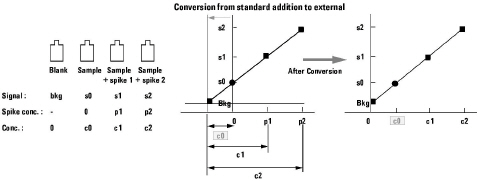
When the signals of sample and spiked solutions are s0, s1 and s2, and the signal of a blank is bkg, the calibration curve obtained by a least squares fit of the points will be as shown below. Using the bkg may be a problem if the sample matrix is quite different from the bkg matrix.

The concentration of analyte added is p1 and p2, and consequently c0 is the concentration of analyte in the sample. When the concentration of the sample is c0, the actual analyte concentrations in the spiked solutions are c1 and c2; e.g. when 10 ppb (p1) and 20 ppb(p2) are added to the sample and the sample concentration is 2 ppb(c0), the actual concentrations of the spiked samples are 12 ppb (c1) and 22 ppb (c2).

 

Method of Standard Additions

Once a standard addition calibration curve is made for one sample, this calibration curve can be converted to an external calibration curve. After conversion, the vertical axis shifts to the bkg point and the point at the concentration of the background becomes the y-intercept. The concentration of the background becomes 0 and the concentrations of other points are recalculated relative to the background; concentrations of other points are combined values of spiked sample concentrations and sample concentrations. After the conversion, the calibration point of a 10 ppb spiked solution becomes 12 ppb when using the above example. The calibration table is also updated according to the calibration curve.

If the matrix of other samples is similar to the first sample, the converted external calibration curve can be used.

 

The method of standard additions should not be used for an analyte that has significant polyatomic interference, since it is impossible to know what part of the signal in the sample is due to analyte, and what part is due to an interference.

 

Curve Fit

• Linear : Select this type when the approximation formula for the plotted calibration curve fits a linear formula (y = ax + b). Normally select this type.
• Quadratic : Select this type when the approximation formula for the plotted calibration curve fits a quadratic formula (y = ax2 + bx + c).
• Avg. RF： Select this item when an average response factor is used to perform quantitation.
• Excluded : Select when the sample is to be excluded.

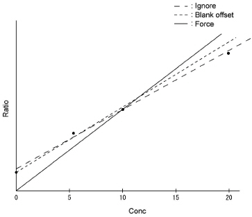
Origin

• Ignore origin: The origin is not included in the calibration curve.
• Force through origin: Forces the calibration curve to pass through the origin.
• Force through blank: Forces the calibration through the blank. (Default)

 

VIS (Virtual Internal Standard) correction

1 Definition of Virtual Internal Standard

The latest revision of ICP-MSICP-QQQ MassHunter Workstation includes a function that allows the internal standard correction factor that is applied to a given analyte to be calculated from the actual signal change of one or more of the internal standards, based on the relative mass of the internal standards and the analyte. This can improve the accuracy of the internal standard correction factor applied, particularly when available internal standards are widely separated in mass and when long-term drift occurs for a component that is mass-dependent.

 

The VIS correction is not supported for an MS/MS scan. It is supported only for a Single Quad scan.

 

2 How to use

1 Background

The main reason for the use of internal standards in ICP-MSICP-QQQ is to correct for long-term drift, which results from changes to the characteristics of the interface cones. Small changes to the profile of the sample cone orifice can occur after a prolonged period of analyzing high dissolved solids samples. The fact that this signal drift is sometimes different for different analyte masses means that several internal standards should be used to accurately correct for the signal drift. In cases where the analytes are many mass units away from the nearest internal standard, or a limited number of internal standards are available, the accuracy of the correction can be improved by using interpolation of the drift correction factor between the measured internal standard elements.

In addition to the accurate correction of mass-dependent drift, interpolation of internal standards can be used to correct for some aspects of matrix effects, since space charge is one of the biggest contributions to the matrix effect. In this case we might expect to observe some mass dependency of the matrix effect, similar to that observed due to drift caused by some heavy matrix introduction. Virtual Internal Standard correction may also be used to correct for matrix effect, where the main component of the matrix effect is mass dependent, particularly when available ISTDs are limited. Because this is an optional function, you should confirm that this option works well for your analysis.

2 Effective Example

 

Drift Change & Matrix Effect Dependence on Mass

In this scatter plot Li6, Sc45, Y89, Rh103, In115, Tb159 and Bi209 show a clear mass dependency. This virtual ISTD correction option is useful, especially when some ISTDs are not available.

3 Limitation

It is important to note that space charge effects are not the only matrix effect. In particular, a high matrix component in the sample is likely to lead to ionization suppression in the plasma, in which case the main component of the signal change is the analyte ionization potential, not the analyte mass. If this is the case, then mass-based interpolation of the internal standard signal will not necessarily improve the data and a better approach would be to select internal standards that are close to the analytes in terms of ionization potential. If the relationship between the mass of analytes and the sensitivity change is not consistent, then use the Virtual Internal Standard correction option with caution. The ISTDs behavior on mass axis can be checked easily and, if necessary, you can make a further detailed check by a recovery test.

VIS compensation formula

The VIS compensation formula is used by selecting how to utilize the VIS element to calculate the VIS. The VIS element refers to the Internal Standard Element used to calculate the VIS (Virtual Internal Standard). This can be set by marking the VIS Flag for the element.

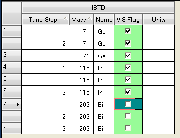
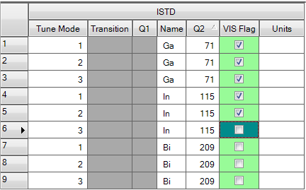
VIS Flag

In the example shown above, Ga and In are set as VIS elements. By selecting Point-to-Point, MassHunter will draw a virtual line connecting Ga and In. This virtual line places a VIS along the line for the elements in each mass between the two points, and is used to calculate the internal standard for each element.

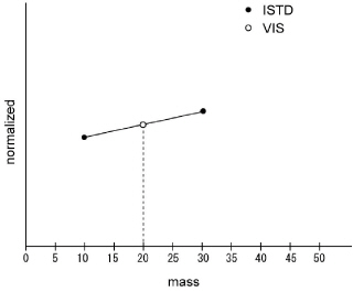
Point-to-Point

Requires one or more VIS elements. Note, if there is only one VIS element, the results are the same as a normal internal standard correction. To use VIS correction, always specify two or more VIS elements. VIS is calculated by connecting two or more elements with a straight line.

 

Point-to-Point

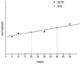
Linear

MassHunter calculates the VIS using a linear equation created from all VIS element data. Requires at least two VIS elements.

 

Linear

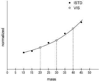
Quadratic

MassHunter calculates the VIS using a quadratic equation created from all VIS element data. Requires at least three VIS elements.

 

Quadratic

Calibration curve weighting

Generally, weighting is turned on when a low concentration is quantitated using a calibration curve with a wide dynamic range. When weighting is turned on, the calibration curve is drawn with weighting applied to a lower standard deviation (SD) level. The calibration curve is calculated based on the standard deviation SD at each concentration level. In other words, the calibration curve is affected more by a high-SD level. Generally, the SD of a high-concentration sample tends to be higher than that of a low-concentration sample. Consequently, calibration without weighting results in a smaller error on the high concentration side and a larger error on the low concentration side.

Therefore, when a low concentration is quantitated using a calibration curve with a wide dynamic range, set weighting to on and draw the calibration curve with a heavier weighting applied to the low concentration side (low SD) than the high concentration side (high SD). When the data used for individual levels contains a different number of replicates, apply weighting to the level with a lower standard deviation (SD) for the drawing of the calibration curve.

 

Weighting

• None: No weighting is applied to the calibration curve.
• 1/x: If the error increases as the concentration increases, select this weight to lower the influence of high concentration samples.
• 1/yx: If the error increases as the strength ratio increases, select this weight to lower the influence of high strength ratio samples.
• 1/SD^2: If the standard deviation error is excessive during replicated measurement, select this weight to lower the influence.
• 1/x^2: Select this weight to lower the influence further compared to the 1/x weight.