Internal Standard Method and Standard Addition Method

Internal Standard Solution

This method is recommended in the following cases:

• When measuring samples with a high matrix concentration.

  When the total matrix concentration exceeds 100 ppm in, for example, sewage or environmental water. In such cases, there are non-spectroscopic interferences. They are physical effects which occur in the plasma and the center chamber region of the instrument which affect the analyte signal in a non-specific way. Typically, the result is suppression of signal across a range of masses or sometimes across a range of ionization potentials. For example, very high concentrations of high mass matrix elements can suppress lower mass elements via space charge effects. Lighter mass ions are repelled from the ion beam by the presence of heavier ions.

  These interferences can be also corrected by the method of standard additions.

• When measurement takes a long time due to large numbers of samples, internal standardization adjusts for sensitivity drift.

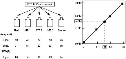
  This is the method by which the analyte signal drift is corrected by the signal of another element (the internal standard element), which is added to both the standard solution and the sample. If the signal of the analyte is affected for any of the above reasons, the internal standard element should be affected in the same way, therefore the ratio of analyte to internal standard element is not affected (see below).

  When the signals of blank, standard solution and sample are a0, a1, a2, a3, and as, and the signals of internal standard in each solution are b0, b1, b2, b3 and bs, then the vertical and horizontal axes of calibration curve are the a to b ratio and the concentration as shown below. When the ratio of sample is as/bs, the concentration of sample (cs) can be calculated according to the calibration curve.

   

  Internal Standard Method

In the calibration report or the calibration graphs, the ratio of the analyte to internal standard is given, not the counts.

Matrix effects are not normally an issue with drinking water, but the use of internal standards is recommended if the water hardness is high. The method of standard additions can also be used for this purpose.

• Selecting internal standard elements

  Since the analytes and internal standard elements should show the same behavior, the internal standard elements should be selected to have mass numbers and/or ionization potentials similar to the analytes: e.g. Bi (209 AMU) is a good internal standard for the measurement of Pb (208 AMU) because of the proximity in mass number, and Zn (9.39 eV) is good for measurement of Cd (8.99 eV) because of its similar ionization potential.

  As a rule, elements that are not originally present in the sample should be selected. However, an element that is present in the sample might be used when the quantity of the element is sufficiently small compared to the signal of the added internal standard. As a guide, semiquantitative analysis should be done first to determine which elements are present in a sample. Elements that are commonly used as internal standards are Li, Be, Sc, Co, Ga, Rb, Y, Rh, In, Cs, Ce, Tl and Bi.

  • EPA Method 200.8

    Li6 amu, Sc , Y , Rh , In , Tb , Ho , Lu , Bi

  • EPA Method 6020

    Li6 amu, Sc , Y , Rh , In , Tb , Ho , Bi

    Note that Li may be present in environmental samples, therefore a solution artificially enriched in ⁶Li is recommended, although it is expensive.

• Concentration of internal standards

  When the internal standard elements are directly added to the sample and standard solutions, the concentration of each internal standard element after addition should be the same in both the sample and the standard solutions used to produce the calibration curve. In addition, the concentration of internal standards in the standard solution at level 1 (the calibration blank in the calibration table) and that in the samples must be the same and must not be 0.

  When the peristaltic pump is used for on-line introduction of an internal standard, the internal standard solution must be prepared separately from the sample and the calibration curve standard solutions. The inner diameter of the internal standard introduction tubing is much smaller than the inner diameter of the sample introduction tubing and so the uptake rate of the internal standard solution is about 1/20 of the sample uptake rate. The internal standard solution is about 20 times less than the sample, and therefore the internal standard solution must be prepared with a higher concentration; ISTD (example for 7700xx-lens7900x: Be (2 ppm), Ga (50 ppb), In/Tl (200 ppb)) is normally appropriate.

• Measurement

  The internal standard elements must be selected in the acquisition parameters as well as the analytes. An integration time of 1 to 3 seconds per element is recommended. Since the inner diameter of the internal standard tube is small, it can take extra time to get a stable signal due to analyte adsorption, so that the first analysis must be started 3 minutes after the signal of the internal standard element appears. In general, longer stabilization times are required for on-line internal standard addition.

Standard Addition to a Sample

This method is recommended to correct matrix effects such as signal suppression or enhancement. A standard solution is directly added to a sample. Since a small amount of the standard solution is added to the sample, the matrix effect is the same for both the sample and the standard. This effect can be used to correct for signal suppression or enhancement.

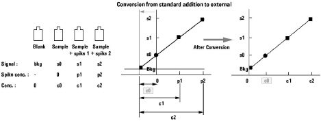
When the signals of sample and spiked solutions are s0, s1 and s2, and the signal of a blank is bkg, the calibration curve obtained by a least squares fit of the points is shown below. Using the bkg may be a problem if the sample matrix is quite different from the bkg matrix.

The concentration of analyte added is p1 and p2, and consequently c0 is the concentration of analyte in the sample. When the concentration of the sample is c0, the actual analyte concentrations in the spiked solutions are c1 and c2; e.g. when 10 ppb (p1) and 20 ppb(p2) are added to the sample and the sample concentration is 2 ppb(c0), the actual concentrations of the spiked samples are 12 ppb (c1) and 22 ppb (c2).

 

Method of Standard Additions

Once a standard addition calibration curve is made for one sample, this calibration curve can be converted to an external calibration curve. After conversion, the vertical axis shifts to the bkg point and the point at the concentration of the background becomes the y-intercept. The concentration of the background becomes 0 and the concentrations of other points are recalculated relative to the background; concentrations of other points are combined values of spiked sample concentrations and sample concentrations. After the conversion, the calibration point of a 10 ppb spiked solution becomes 12 ppb when using the above example. The calibration table is also updated.

If the matrix of other samples is similar to the first sample, the converted external calibration curve can be used.

• Concentration of standard solutions

  The concentration of each element after addition to the sample should be of the same order (preferably half to 2X) the original concentration in the sample. If the concentration of the standard and the original concentration of the sample are very different, the calculation error will be significant.

• Measurement

  If a signal contains some background such as random background and/or memory from the sample introduction system, it may also be calculated as the analyte concentration contained in the sample, which might cause a quantitation error. To avoid that, the measurement of pure water or nitric acid diluted with pure water is recommended and used as the background file.

  If you analyzed a blank solution as a background, select the data in the same way as the other sample's data when you create calibration curves. Enter "-1" or "b" for the concentration in the calibration curve table. ("Bkg" is displayed in the screen.)

  In the standard addition method, quantitation results are obtained at the time a calibration curve is created. You can see the quantitation value in the plot of the calibration curve. If you wish to output only the quantitation result, use Quantitation Report as in the case of the normal results. Here, since the quantitation result is a part of the method, if you select a calibration curve for the standard addition method, the quantitation result of the samples used for the calibration curve is output regardless of the file that is loaded on the data analysis screen.