Quantitation

 

MassHunter measures an intensity ratio for each replicate data and averages them to get the final intensity ratio.

 

Internal Standard

When an internal standard is selected in the current calibration curve, the count of the target ion of the sample data is divided by the ratio of the count per concentration of the internal standard in the sample data. In this calculation, the concentration of the internal standard in the first level of the calibration curve is used as the concentration of the internal standard in the sample data. The count value for each element reported on a quantitative report is therefore a count ratio.

y=y_s /(y_i/x_i) (y=y_s if x_i=0)

where

x_i : concentration of the internal standard of the first level in the calibration curve

y_i : count of internal standard

y_s : count of the target ion

This value is used as the measured value of y in the following sections.

Calculating Concentration

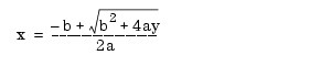
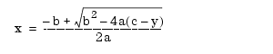
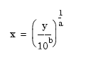
Concentration of the target ion of the sample data is calculated as follows.

where

x: concentration of the target ion

y: measured count of the target ion

a: coefficient "a" in the calibration curve

b: coefficient "b" in the calibration curve

c: coefficient "c" in the calibration curve

1. y = ax

 

2. y = ax + b

 

3. y = ax²+ bx

 

4. y = ax² + bx + c

 

5. log y = a (log x) + b

 

6. y = ax + b + bkg (Standard Addition)

 

7. y = ax + [blank]

    

   where

   blk: number of counts in the calibration blank

Standard Deviation of the Concentration

When a linear regression is used, the standard deviation is calculated as follows.

 

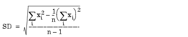
n : number of sample replicates

x_i: concentration

DL

DL refers to a concentration equivalent to 3B.

The equation for DL varies depending on the calibration formula.

If a linear equation such as y=ax+b is used:

DL = 3sB/a

Where, 3B: value three times the standard deviation of the count at the 0 concentration level.

a: a in y=ax+b

The unit set in the calibration should be used and must not be changed.

Interpolation Formulas for Virtual-Internal-Standard Correction

These formulas are used to calculate the modification rates for all internal standards used for the latest calibration curve and the current sample data. The concentration level of the current data internal standards uses the value of level 1 of the calibration curve, as with the existing internal-standard correction. In the case of Linear and Quadratic, one formula is created from all internal-standard modification rates. In the case of Point-to-Point, a formula is created for every two internal standards.

 

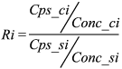
where

Cps_ci, Conc_ci : CPS and concentration of the internal standard of the data last used to update the calibration curve

Cps_si, Conc_si : CPS and concentration of the internal standard of the current sample data (For the concentration, use the value set for level 1 of the calibration curve.)

Point to Point (Y = aX + b; Two adjacent internal standards are used; Default)

Linear (Y = aX + b; All internal standards are used.)

 

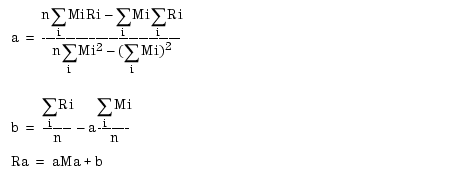
where

Mi : Mass number of internal standards

n : Number of internal standards (two in the case of "Point to Point")

Ri : Modification rate of the internal-standard CPS between the standard data and sample data

Ma : Mass number of the element to be quantified

Ra : Virtual-internal-standard correction coefficient for correcting the CPS of the element to be quantified

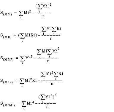
Quadratic (Y = aX²+bX+c ; All internal standards are used.)

 

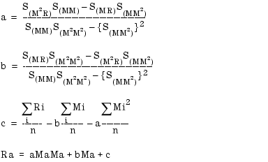
where

Mi : Mass number of internal standards

n : Number of internal standards

Ri: Modification rate of the internal-standard CPS between the standard data and sample data

Ma : Mass number of the element to be quantified

Ra: Virtual-internal-standard correction coefficient used to correct the CPS of the element to be quantified

 

Correct the CPS of the element to be quantified using the virtual-internal-standard correction coefficient.

Cps_na = Cps_saÞRa

where

Cps_na : Corrected CPS of the element to be quantified

Cps_sa : CPS of the element to be quantified

Ra : Virtual-internal-standard correction coefficient for the CPS of the element to be quantified

REE++ Correction

Signals that interfere with X are calculated as,

 

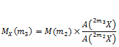
where A(μ) is the abundance of μ, M(μ) is the signal of μ, and mi is the m/z of M++ for X. μ is the isotope of the interfered element.

The coefficient, , is defined as,

 

And is,

 

The corrected signal, , is calculated as,

 

Refer to the following table for each parameter:

Correction for 75 As			Correction for 78 Se			Correction for 66 Zn
X	M++	Abd.	X	M++	Abd.	X	M++	Abd.
Nd	m3: 75	5.6	Gd	m3: 78	20.47	Ba	m3: 66	0.1
	m2: 72.5	8.3		m2: 77.5	14.8		m2: 67.5	6.59
Sm	m3: 75	7.38	Dy	m3: 78	0.06
	m2: 73.5	14.99		m2: 81.5	24.90

This correction is applied to only FullQuant analysis. This is not applied to SemiQuant analysis and other analysis modes.