Setting up a Chromatographic Data Analysis Method using the Optional Chromatographic Software Module
New features in MassHunter 4.2 make creating and calibrating a chromatographic data analysis method easier than ever.
As the first step, you need to acquire a set of calibration standards and ensure that the resolution, sensitivity, peak shape, baseline etc. are acceptable. In general, this can be verified visually.
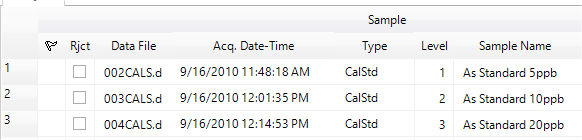
If you are working with a previously acquired batch of samples, you can open the batch using Offline Data Analysis by clicking [Open Folder] from the [Batch] group on the [Home] tab, and selecting the batch from the list. The list of samples in the batch is displayed in the Batch at a Glance table.
Ensure that the calibration standards are designated as sample type “Calstd” in Data Analysis. If they were originally acquired as sample type “Sample” during acquisition, change the sample type in the Batch View Grid. You do not need to include a Calblk in chromatographic analysis. The lowest concentration standard should contain recognizable peaks for all analytes.
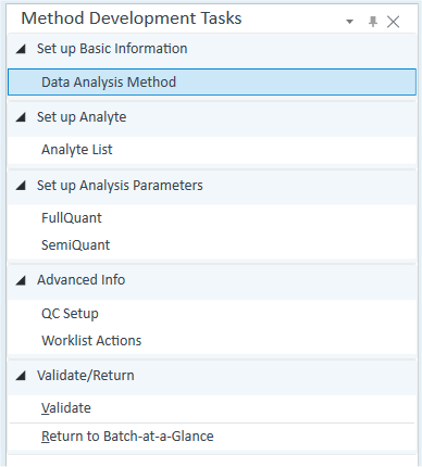
- Click [Edit] from the [Method] group on the [Home] tab.

The [Method Editor] window is displayed.
- In the Method Development Tasks Pane, click [Open Data File…],
and then select a calibration standard data file with good quality
peaks (a mid-range standard is a good choice).
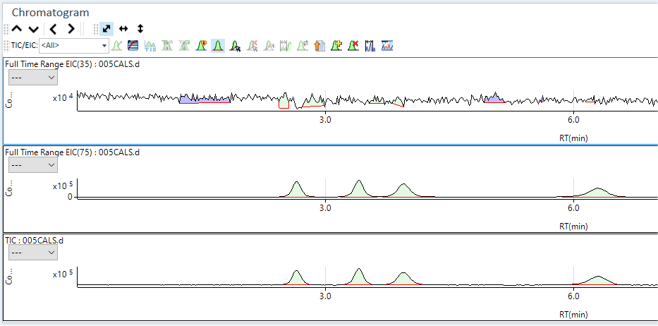
The total ion chromatogram (TIC) for the selected calibration standard data file is displayed as shown below. If your acquisition includes more than one element or isotope and internal standards, the baseline may look noisy and the peaks may appear smaller than expected because you are seeing a composite of all signals.
- Pull down the list box that currently shows TIC (circled) and select
the mass for the first group of analytes that you want to enter into
your method.
For example, if you are looking for arsenic compounds, select mass 75.
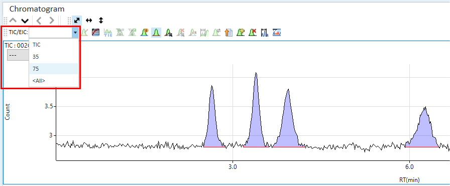
The integrated extracted ion chromatogram (EIC) for the selected mass is displayed.
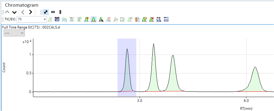
If your method includes compounds or species of different elements, then select <All> from the TIC/EIC menu to display all acquired EICs and the TIC simultaneously. This allows you to add all your selected analyte peaks from different masses to the peak list table graphically. You may need to enlarge the Chromatogram window to see all of the EIC traces clearly if there are more than 2-3. In the example below, the only analyte is As at m/z = 75. However, m/z 35 was included to indicate the presence of interferences from ArCl due to Cl containing peaks.
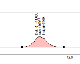
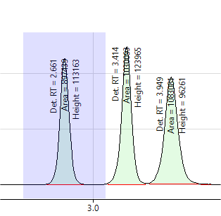
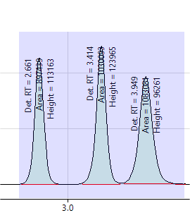
- If all of the peaks are not correctly integrated using the default
integration parameters, as shown below, click
 on the manual integration tool and draw in the correct baseline.
The manually integrated peaks are red.
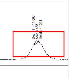
Before manual integration above; after manual integration below.
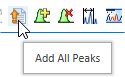
- After all peaks are correctly integrated, you can add these compounds
to the Peak List by using the “Add All Peaks” tool.
The integrated peaks are added to the Peak list in order of retention time.
Alternatively, you can choose individual peaks from each EIC to add to the Peak Table by using the “Add Peak Mode” tool
 .
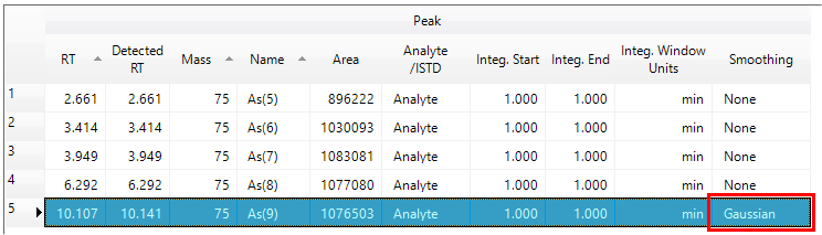
.At this point, you can edit the peak table to change the compound names, designation as analyte, or internal standard and target or qualifier ion. If the auto-integration process did not correctly, integrate a peak (in this example peak 5 was incorrectly integrated due to a noisy apex), select the Smoothing column for the noisy peaks, and then turn on Gaussian smoothing.
- Once the peaks are added, you can step through them one by one
by clicking on them in the table and view the default integration
windows in the chromatogram display.
The windows should be wide enough to easily capture the peak start and end, but not so wide as to contain several peaks (if possible). Adjust the integration windows as needed by changing the “Integ Start” and “Integ End” values in the Peak Table. The graphic below on the left shows a correctly set integration window for peak 1. The graphic on the right shows an integration window for peak 2 that is too wide.
- Once all desired peaks are correctly integrated and added to the peak list with the correct information filled in, Click on “FullQuant” under the Method Development Tasks pane on the left of the screen.
- Fill in the calibration and QC information as shown below. You
may or may not have spike samples or QC samples. If not, these columns
can be left blank. For more information about completing various QC
samples information, refer to the training module “Understanding QC
Error Action Functions”.

- Click [Validate] near the bottom of the Method Development Tasks Pane to check for any errors and correct them if necessary.
- Click [Return to Batch-at-a-Glance] at the bottom of the pane,
to return to the Batch View. Click [Yes] to the “Update Data Analysis
Method?” question.
Results are displayed for the entire batch via the Batch at a Glance Table at the top, and graphically for each sample at the bottom. Click individual samples and/or peaks from the table to select them. The Chromatogram pane shows the EIC for the entire run on top, and the selected analyte peak on the bottom. If the baseline on the target ion (bottom chromatogram trace) indicates incorrect integration, use the manual integration tool
 to correct
the integration. The [Process Batch] icon changes to
to correct
the integration. The [Process Batch] icon changes to  .
Click this icon to requant the batch including your manually integrated
peaks.
.
Click this icon to requant the batch including your manually integrated
peaks. - When you are satisfied with your results, click [Save Batch Results] from the [Batch] group on the [Home] tab.