Single Nanoparticle Application (Option)

This section describes the procedures for performing data analysis and checking the analysis results with the optional Single Nanoparticle application.

• Acquiring data for Single Nanoparticle Analysis
• Analyzing data for Single Nanoparticle Analysis
• Particle Size Distribution Pane Operations
• Single Particle Method Editor Pane Operations

Acquiring data for Single Nanoparticle Analysis

To acquire data for single nanoparticle analysis, refer to "Analyzing Single Nanoparticles using the Optional Single Nanoparticle Application Module" under "Workflow".

Analyzing data for Single Nanoparticle Analysis

This section explains how to analyze data for single nanoparticle analysis.

Processing data

After completing measurements, run an analyzing process from the [Data Analysis] window. To do this, follow the steps below:

1. Click [Process Batch] from the [Batch Option] group on the [Home] tab.

   Analysis is performed using the settings in the Data Analysis Method, and the batch results are displayed in the [Batch Table] pane.

    

Reviewing results from the Batch Table pane

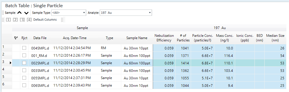
For a Single Particle Analysis, different titles than those of a normal FullQuant Analysis are displayed for the [Analyte] columns in the [Batch Table] pane as shown below:

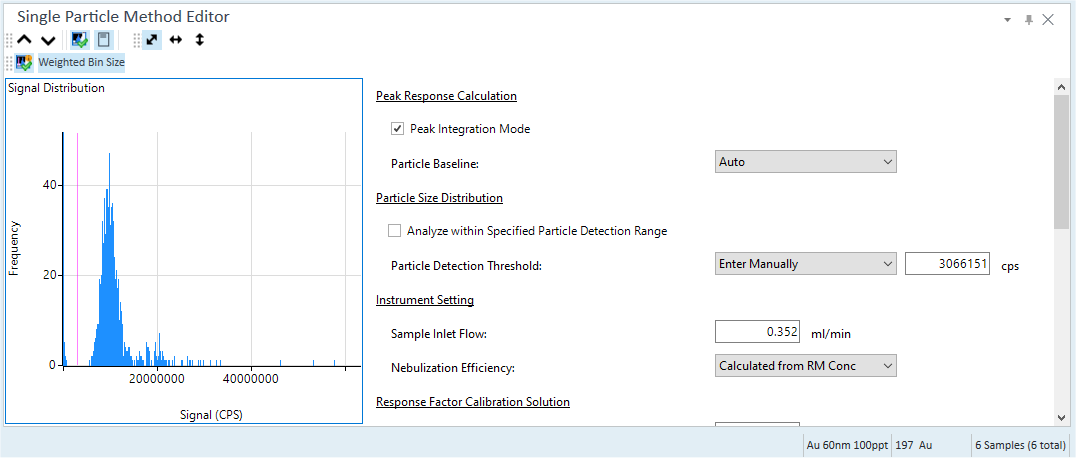
• Nebulization Efficiency column

  Nebulization Efficiency is calculated as follows:

   

• # of Particles column

  Displays the Number of detected particles.

• Particle Conc. (Particles/l) column

  Displays the particle number per 1 liter.

• Mass Conc. (ng/l) column

  Displays the mass (ng) of particles per 1 liter.

• Median Size (nm) column

  Displays the median particle size (nm).

• Ionic Conc.(ppb) column

  Displays the dissolved ionic concentration.

• BED column

  Displays the Background Equivalent Diameter. (BED) which permits an estimation of the approximate minimum particle size detection limit and aids in the selection of the detection threshold.

• Mean Particle Signal column

  This indicates the average calculated from signals over [Particle Detection Threshold] and within a specified [Particle Detection Range].

• Mean Size (nm) column

  Displays the mean particle size (nm).

• Most Freq. Size (nm) column

  Displays the particle diameter (mm) of the particle with the highest frequency.

• NP Ratio column

  Displays the intensity ratio of two Isotopes when analyzing two isotopes in a single particle.

• Particle Baseline column

  Displays the Particle Baseline (CPS).

• FullQuant Signal (CPS) column

  Displays the CPS of the respective analyte element(s) using FullQuant analysis based on the mean signal value of the TRA data over the specified range.

• FullQuant Conc. (ppb) column

  Displays the concentration of the respective analyte element(s) using FullQuant analysis of the FullQuant signal (CPS) divided by the element response factor (CPS/ppb).

• Mean Mass (ag) column

  Displays the mean mass of analyte element per particle (atto gram = 10^-18 gram).

• Median Mass (ag) column

  Displays the median mass of analyte element per particle (atto gram = 10^-18 gram).

• Most Freq. Mass (ag) column

  Displays mass of analyte element per particle with the highest frequency (atto gram = 10^-18 gram).

• Particle Detection Threshold column

  The limit value (CPS) that separates particles from noise and ions.

• FullQuant Meas. Conc. (ppb) column

  Displays the concentration of the measured data. Displays the concentration for each element to which the dilution factor is not applied.

 

• When you open Single Nanoparticle Analysis batches, the following concentrations are calculated using the Total Dilution factor:

• Particle Conc.  (particles/l)

• Mass Conc. (ng/l)

• Ionic Conc. (ppb)

• FullQuant Conc. (ppb)

  (FullQuant Meas. Conc. is calculated without the dilution factor.)

• In Data Analysis, the Total Dil. column is available. IonicBlk, IonicStd(AN), IonicStd(RM), and RM are disabled. This means the dilution factor should always be 1.0.

 

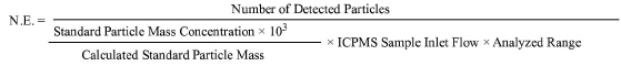
Reviewing results from the Particle Size Distribution pane

The Time Scan chart and the Particle Size Distribution currently selected in the [Batch] table can be reviewed from the [Particle Size Distribution] pane.

 

For details on the operations, refer to the "Particle Size Distribution Pane (Option)".

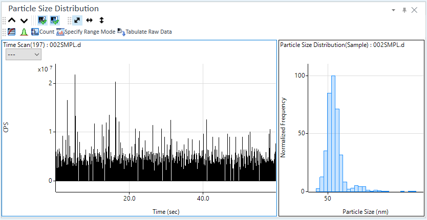
Reviewing results from the Single Particle Method Editor pane

For Single Particle Analysis, use the [Single Particle Method Editor] pane to modify the Data Analysis Method. The Single Particle Method Editor pane will be displayed by default in the lower right of the Window.

 

The [Method Editor] window will not be available as it usually is in FullQuant Analysis. Use the Single Particle Method Editor instead of the usual Method Editor.

 

 

Parameters

All the parameters for the single particle analysis are displayed here. Parameters which have been set in the Method Wizard are shown as default and these can be modified as required.

Signal Distribution

The Signal Distribution currently selected in the Batch table can be reviewed. Particle Detection Threshold can be set by left clicking within this view, as well as inputting the value directly in the 'Particle Detection Threshold' column.

Refer to "Single Particle Method Editor Pane (Option)" for an explanation of the icons and functions available in the toolbar of this pane.

Reprocessing data

If you change the Data Analysis Method, the [Process Batch] icon changes to . Click the icon to start an analysis process.

Saving the batch results

This process saves batch results.

To save batch results, click [Save] from the [Batch] group on the [Home] tab.

Particle Size Distribution Pane Operations

This section explains how to use the Particle Size Distribution Pane (Option) which is displayed when you analyze samples using the optional Single Nanoparticle Application.

For information about functions that are common to all panes, refer to "Common Pane Operations".

 

Displaying the Particle Size Distribution Pane

This pane displays the Time Scan data and the calculated Particle Size Distribution charts for the current focused sample in the Batch Table.

Time Scan Chart

Displays the Time Scan Chart for the sample selected in the Batch Table.

Toggling between Count view and CPS view

You can toggle between Count view and CPS view by turning on [Count] in the toolbar.

Specify Range Mode

You can select the time range visually in the Time Scan Chart for calculation of particle size distribution by turning on [Specify Range Mode] in the toolbar. The selected range is indicated by a purple-colored rectangle on the Time Scan Chart. Even if this button is unavailable, the selected time range is used to perform calculations. The default range is the entire range of the raw data on the Time Scan Chart.

Particle Size Distribution Chart

Displays the Particle Size Distribution Chart calculated from the Single Particle Analysis.

Toolbar Functions

For more information on the toolbar functions, refer to the "Particle Size Distribution Pane (Option)".

Adjusting the scales

You can change the scales for the X- and Y- axes. For more information, refer to "Adjusting the scales" under "Common Graph Operations".

Shifting the axes

You can switch the X- and Y- axes. For more information, refer to "Shifting the axes" under "Common Graph Operations".

Adding comments

For more information on adding/deleting comments, refer to "Adding comments".

Tabulating raw and CPS data

You can create a CSV format table based on the raw or CPS data for the chart. For more information, refer to "Tabulating raw and CPS data".

Copying charts

You can copy charts to the Clipboard and then paste them into documents created with other applications. For more information, refer to "Copying the graphs" under "Common Graph Operations".

Printing charts

You can print charts. For more information, refer to "Printing the panes" under "Common Pane Operations".

Exporting charts

You can export charts in various graphic file formats. For more information, refer to "Exporting the graphs" under "Common Graph Operations".

Single Particle Method Editor Pane Operations

This section explains the operations for the Particle Size Distribution Pane (Option) which is displayed when you analyze samples with the optional Single Nanoparticle Application.

For information about functions that are common to all panes, refer to "Common Pane Operations".

 

Displaying the Single Particle Method Editor Pane

This pane displays the Method Editor that allows you to display and change each parameter for the Signal Distribution chart and the Single Particle Analysis in samples selected from the Batch Table.

• Signal Distribution chart
• Method Editor

Signal Distribution chart

This is calculated from the raw data for the current focused sample in the Batch Table.

Toolbar Functions

For more information on the toolbar functions, refer to the "Single Particle Method Editor Pane (Option)".

Adjusting the scales

You can change the scales for the X- and Y- axes. For more information, refer to "Adjusting the scales" under "Common Graph Operations".

Shifting the axes

You can switch the X- and Y- axes. For more information, refer to "Shifting the axes" under "Common Graph Operations".

Tabulate Chart Data to CSV

Exports the "Frequency Vs signal" data to a CSV file, and then opens the CSV file.

1. Right-click on the Signal Distribution chart.

   The context menu is displayed.

2. Select [Tabulate Chart Data to CSV].

3. The associated application starts, and the "Frequency Vs signal" table is displayed.

Copying charts

You can copy charts to the Clipboard and then paste them into documents created with other applications. For more information, refer to "Copying the graphs" under "Common Graph Operations".

Printing charts

You can print charts. For more information, refer to "Printing the panes" under "Common Pane Operations".

Exporting charts

You can export charts in various graphic file formats. For more information, refer to "Exporting the graphs" under "Common Graph Operations".

Method Editor

Displays each parameter for Single Particle Analysis and allows you to make changes. For more information, "Method Editor".