Batch Table Pane Operation
This section explains the operation of the Batch Table pane.
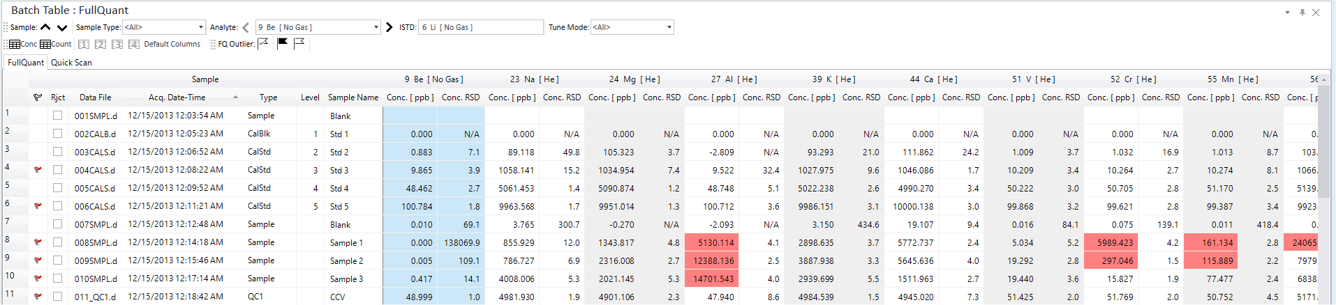
The Batch Table pane displays sample information and data analysis results. The example below uses FullQuant Analysis to show you how to use of the Batch Table pane.
For the information about the functions of this pane, refer to “Batch Table pane”.
For more information on the functions that are common to all panes, refer to “Common Pane Operations”.
Batch Table Pane
Switching the sample display setting
Displaying by calibration curve groups
Toolbar Functions
For the information about the functions of the toolbar, refer to “Batch Table pane”.
Changing the layout
The Batch Table has two layout views: “Simple” and “Detail”. You can change the by selecting [Batch Table Layout] - [Detail] or [Simple] from the [Batch Table] group on the [View] tab.
- Simple
You can select the rows to be displayed for this layout. (Default)
In Table mode, you can change the columns to display by selecting [Adding/Removing Columns]. For details, refer to “Adding/Removing columns” under “Customizing columns”.
Note that on the toolbar, clicking [Concentration] displays the Concentration view, and [Count] displays the Count view.
- Detail
Detailed data for each sample is displayed.
- Add/Remove Columns
When [Simple] is selected, you can specify the columns that are displayed in the batch table.
For data measured by an MS/MS scan, the [Scan Type], [Transition], [Q1], and [Q2] columns are displayed.
Loading a batch result
To load the data file into the Batch Table pane, open a Batch Folder and load a batch result. When performing a new data analysis, create a new Batch Folder.
Creating a batch folder
Before you perform a new data analysis, you will need to create a new Batch Folder for storing the analysis results. To create a new Batch Folder, follow these steps:
When using ECM, OpenLab Server Products, Workstation Plus, or SDA, the displayed dialog box and the save file destination differ from standard MassHunter operations. For more information, refer to " Operations When Database Systems Are Used" in "Reference".
- Click [New Batch Folder] on the [File] tab and click [Browse].
The [New Batch Folder] dialog box appears.
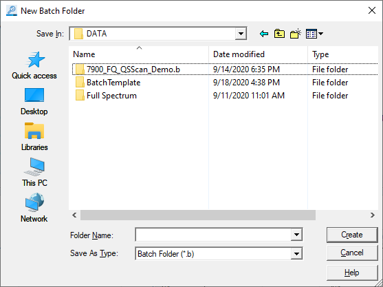
[New Batch Folder] Dialog Box
- Open the folder to create the Batch Folder in, enter the folder
name into the [Folder Name] text box, and click <Create>.
The Batch Folder for storing the analysis results files is created.
Loading a batch result
To open an existing Batch Result, follow these steps:
When using ECM, OpenLab Server Products, Workstation Plus, or SDA, the displayed dialog box and the save file destination differ from standard MassHunter operations. For more information, refer to " Operations When Database Systems Are Used" in "Reference".
- Click [Open] from the [Batch] group on the [Home] tab.
The [Open Batch Result] dialog box is displayed.
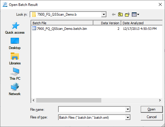
[Open Batch Result] Dialog Box
- Select the Batch Result, and click <Open>.
The selected data is displayed in the [ICP-MSICP-QQQ Data Analysis] window.
Loading acquired data
This section describes how to load the acquired data into the Batch Table pane. You can load all acquired data from within a Batch Folder, or load only the selected data from a data folder.
You cannot load data for other analysis modes.
When using ECM, OpenLab Server Products, Workstation Plus, or SDA, the displayed dialog box and the save file destination differ from standard MassHunter operations. For more information, refer to " Operations When Database Systems Are Used" in "Reference".
Loading data from a different batch folder
To load the acquired all data from another existing Batch Folder (*.B), follow these steps:
When using ECM, OpenLab Server Products, Workstation Plus, or SDA, the displayed dialog box and the save file destination differ from standard MassHunter operations. For more information, refer to " Operations When Database Systems Are Used" in "Reference".
- Click [Import Samples] - [Import All Samples from Batch] from the
[Batch] group on the [Home] tab.
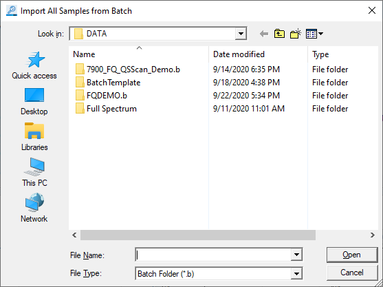
The [Import All Samples from Batch] dialog box is displayed.
[Import All Samples from Batch] Dialog Box
- Select a batch folder (*.B), and click <Open>.
The acquired data is loaded into the current Batch Table.
Loading data from a data folder
To load the acquired data from a data folder (*.D), follow these steps:
When using ECM, OpenLab Server Products, Workstation Plus, or SDA, the displayed dialog box and the save file destination differ from standard MassHunter operations. For more information, refer to " Operations When Database Systems Are Used" in "Reference".
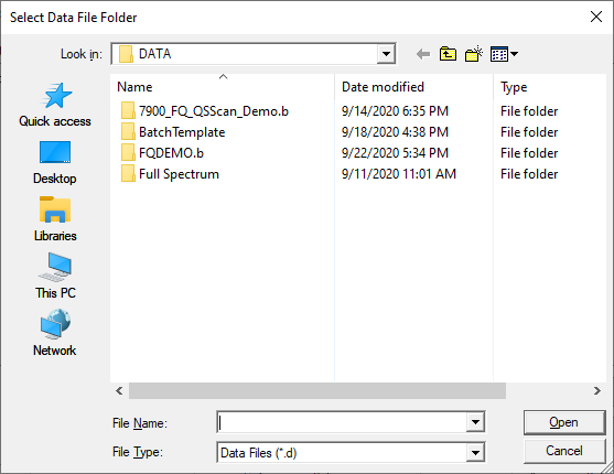
- Click [Import Samples] - [Import Samples] from the [Batch] group
on the [Home] tab.
The [Select Data File Folder] dialog box is displayed.
[Select Data File Folder] Dialog Box
- Select the data folder (*.D), and click <Open>.
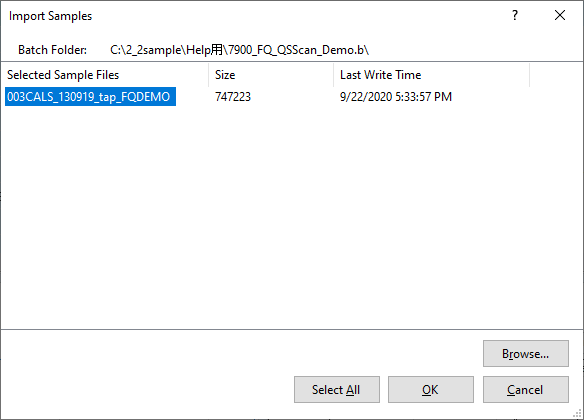
The [Import Samples] dialog box is displayed, and the data files that are contained in the selected folder are listed.
[Import Samples] Dialog Box
- To load additional data files from another folder, click <Browse...>.
The [Select Data File Folder] dialog box is displayed.
Repeat steps 2 and 3 to select multiple data files.
- Select the data file of interest, and click <OK>. (Multiple
selection allowed)
The data is displayed in the current Batch Table pane.
Column Functions
In the Batch Table, each row represents a sample, with the columns displaying information on the samples and elements.
The columns are categorized into four groups: Sample columns, Analyte columns, ISTD columns, and Replicate Data columns.
- Sample Column
Displays information on a sample, such as its name, type, and calibration curve level.
- Analyte Column
Displays information on an analyte, such as its element name, mass, Tune Mode, concentration, count, CPS (count per second), RSD (relative standard deviation %), and detector mode. The types of columns displayed depend on the Data Analysis Method.
- ISTD Column
The header displays information on an ISTD element, such as its element name, mass, and Tune Mode. The columns display information such as concentration, count, CPS (count per second), and ISTD Recovery%.
- Replicate Data Column
The element name, mass, and Tune Mode of the replicated data are displayed in the column headers, and columns are displayed for the concentration and CPS (counts per second) of each replicated data.
Replicate data columns do not appear in the default Table mode.
This section describes columns that are not shown by default. To display these columns, refer to “Adding/Removing columns” under “Customizing columns” in the next section.
The default column settings depend on the Analysis Mode.
The columns in the Batch Table for an isotope ratio analysis are significantly different from other analysis methods. Refer to the “ Isotope Ratio Analysis Column Functions”.
This section explains the content and function of the columns that are displayed in the Batch Table.
Sample Column
Displays information on a sample, such as its name, type, and calibration
curve level. If all of the samples cannot be displayed in the screen,
use the vertical scroll bar to scroll the display. The samples can also
be displayed by selecting  or
or
 on the Batch Table pane toolbar.
The subcolumns are described below.
Leftmost Column
A ![]() is displayed at
the beginning of the selected sample. Click this column to select the
entire row (sample). To select multiple rows (samples), drag the cursor
across this column.
is displayed at
the beginning of the selected sample. Click this column to select the
entire row (sample). To select multiple rows (samples), drag the cursor
across this column.
Drag the bottom edge of this column to resize the column height for the entire Batch Table.
 Column
Displays a ![]() for an outlier.
Place the cursor on the icon for a popup display of information about
the outlier.
for an outlier.
Place the cursor on the icon for a popup display of information about
the outlier.
Outlier Popup
iQ Column
The iQ mark is displayed when interference might occur.
This column is displayed when:
- [IntelliQuant] is selected for [Data] in the SemiQuant pane.
- [iQ Rating] is on.
Detailed information is displayed in a tooltip.
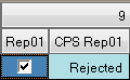
Reject Column
Mark the checkbox for samples that are to be excluded for the data analysis.
Correction Column
The conventional interference correction or REE++ Correction is displayed.
Data File Column
Displays the file name for the data.
Acq Date-Time Column
Displays the date and time at which the data was collected.
Type Column
Displays the sample type. You can also change the sample type by selecting from the list.
Level Column
Displays the calibration curve level. Double-click the column to change the level.
Sample Name Column
Displays the sample name that was entered during data acquisition. Double-click the column to change the sample name.
Total Dil. Column
Displays the total dilution factor. Double-click the column to display the [Calculate Dilution Factor] dialog box, which lets you change the total dilution factor.
For details, refer to [Calculate Dilution Factor] dialog box.
Final Weight or Volume Column
When using Autodilution using ADS 2, the final weight or volume value set in the [Final Weight or Volume] column of the Sample List pane (sequence) is displayed.
To change the value, double-click the Total Dil. Column and change the [Final Weight or Volume] value in the Calculate Dilution Factor dialog box.
Sample Weight or Volume Column
When using Autodilution using ADS 2, the sample weight or volume value set in the [Sample Weight or Volume] column of the Sample List pane (sequence) is displayed.
To change the value, double-click the Total Dil. Column and change the [Sample Weight or Volume] value in the Calculate Dilution Factor dialog box.
Dilution Multiplier Column
When using Autodilution using ADS 2, the dilution multiplier value set in the [Dilution Multiplier] column of the Sample List pane (sequence) is displayed.
To change the value, double-click the Total Dil. Column and change the [Dilution Multiplier] value in the Calculate Dilution Factor dialog box.
Autodilution Column
When using Autodilution using ADS 2, the autodilution factor set in the [Autodilution] column of the Sample List pane (sequence) is displayed. This cannot be edited.
Dilution list Column
When using Autodilution using ADS 2, the elements set in the [Dilution List] column of the Sample List pane (sequence) are displayed. This cannot be edited.
Comment Column
Displays the comment that was entered during data acquisition. Double-click the column to edit the comment.
ISTD Conc Column
Sets the level and concentration of the ISTD. Click the right end of the column to display the [Set ISTD Conc] dialog box, which lets you change the settings. For details, refer to [Set ISTD Conc] dialog box.
Reported Elements Column
Sets whether to include the element in the analysis results report. By default, all elements are included.
This column can be used, for example, to exclude elements that have interference from oxides and doubly charged ions.
Double-click the column and select [All] in the list to include all elements. To exclude an element, clear the element. If the setting has been changed from the default setting, the column will be labeled with <Selected>.
DA Date-Time Column
Displays the date and time that the data was analyzed.
Vial Number Column
Displays the vial number of the sample.
User Define 1/User Define 2/User Define 3 Column
Displays the values that you entered in the [User Define 1]/[User Define 2]/[User Define 3] Column on the Sample List Pane (Sequence).
Acq. Method File Column
Displays the file name of the acquisition method.
%J Column
This is used when you use USP<232>/ICH Q3D method in U.S. Pharmacopeial Convention.
The J value is the concentration (w/w) of the elements of interest at the Target limit, appropriately diluted to the working range of the instrument.
Max. Daily Dose Column
This is used when you use USP<232>/ICH Q3D method in U.S. Pharmacopeial Convention.
By default, the value is empty and does not influence the QC outlier calculations. If a value is assigned, the QC outliers calculated as:
Low Limit £ (Measured Conc × Total Dilution × Max. Daily Dose)/(Reference QC Conc) £ High Limit
SQBlk Column
Is displayed on the [SemiQuant] tab, [Quick Scan] tab, and [IntelliQuant] tab when both the Full Quant and Semi Quant modes are used in analysis.
The SQBlk sample type for the Semi Quant mode can be set for the samples for which the sample type for the Full Quant mode is already set in the Type column. Select the check boxes for the samples you want to set.
SQStd Column
Is displayed on the [SemiQuant] tab, [Quick Scan] tab, and [IntelliQuant] tab when both the Full Quant and Semi Quant modes are used in analysis.
The “CalStd” sample with the highest number of specified elements and the highest calibration curve level is set as the “SQStd” sample.
SQISTD Column
Is displayed on the [SemiQuant] tab, [Quick Scan] tab, and [IntelliQuant] tab when both the Full Quant and Semi Quant modes are used in analysis.
“CalBlk” sample is set as “SQISTD” in "Auto Add" in ISTD Mode.
SQBkgnd Column
Is displayed on the [Quick Scan] tab and [IntelliQuant] tab when both the Full Quant and Semi Quant modes are used in analysis.
- "CalBlk" is set as "SQBkgnd".
- On the [IntelliQuant] tab, you can set the sample type by using the [SQBkgnd] check box.
- The CPS of the latest sample with [SQBkgnd] on is subtracted in the background in the same way as "Bkgnd".
- "SQBkgnd" can only be used with Quick Scan data.
TMS(ppm) Column
You can display the Total Matrix Solids (TMS) column in a batch table on the [FullQuant] tab or the [SemiQuant] ([Quick Scan]/[IntelliQuant]) tab. The value is calculated only when IntelliQuant is set to On.
TMS is calculated as,
![]()
Where, Ci is the concentration of element calculated by IntelliQuant with enough CPS (over the minimum CPS). The unit for the calculated TMS is ppm.
Except for the following:
H, He, C, N, O, F, Ne, P, S, Cl, Ar, Br, Kr, I, Xe, At, Rn
Analyte Column
Displays the analysis results for an analyte. The column headers display the mass, analyte name, and Tune Mode. After an analysis is performed, the concentration and the count for each Tune Mode is displayed for the elements in the sample. For replicate analyses, the average values are displayed. The types of columns that are displayed depend on the Data Analysis Method.
If all of the elements cannot be displayed in the screen, use the horizontal scroll bar to scroll the display.
The hidden analytes can also be displayed by using 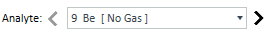 on
the Batch Table pane toolbar.
on
the Batch Table pane toolbar.
The subcolumns are described below.
The column that can be selected is different for a detail mode.
Conc. Column
Displays the concentration of the element.
The iQ mark is displayed when interference might occur.
This mark is displayed when:
- [IntelliQuant] is selected for [Data] in the SemiQuant pane.
- [iQ Rating] is on.
- The rating on the [iQ Rating] tab in the IntelliQuant pane is 3 or less.
Detailed information is displayed in a tooltip.
Conc. RSD Column
Displays the RSD (relative standard deviation %) for the concentration of the element. (Spectrum/Timechart)
Area Column
Displays the peak area when the Analysis Mode is set to “Chromatogram”.
Blk. Conc. Column
Displays the blank concentration.
CPS Column
Displays the CPS (count per second).
CPS RSD Column
Displays the RSD (relative standard deviation %) for the CPS. (Spectrum/Timechart)
Meas conc. Column
Displays the concentration of the measured data. Displays the concentration for each element to which the dilution factor is not applied.
Spike Recovery % Column
If the sample contains “Spike” or “Spike Ref” sample type, the Spike Recovery % value is displayed.
Spike Recovery % is calculated as shown below.
Spike Recovery % = (Diluted Spike Sample's Conc - (Diluted Spike Ref's Conc)/Spike Amount×100
Spike Conc. Column
Displays the concentration of the Spike sample that is used for the recovery check.
Spike Amount Column
Displays the Spike Amount to calculate the Spike Recovery %.
Ratio Column
Displays the intensity ratio of the ISTD.
Det. Column
Displays the detector mode (pulse or analog).
CF Formula Column
Displays the calibration curve equation.
Min Conc. Column
Displays the minimum concentration to be reported.
When a Dilution Factor is set, the Dilution Factor is applied to Min Conc.
CIC Column
Displays the settings for the CIC. (Chromatogram)
Quant by Height Column
When quantifying using the height, a check mark is displayed. (Chromatogram)
RT Column
Displays Retention Time. (Chromatogram)
Height Column
Displays the peak height when the Analysis Mode is set to “Chromatogram”.
Qualifier Ratio Column
Displays the ratio of the qualifier ion relative to the target ion. (Chromatogram)
S/N Column
Displays the S/N ratios for the peaks if the noise range is set. (For chromatograms only) For more information, refer to “Setting the noise range”.
Delta RT Column
Displays the delta RT when the Analysis Mode is set to "Chromatogram". The delta RT can be calculated using the following equation:
Delta RT = Measured RT value - Expectation value of RT
DL Column
This item is displayed in the following cases.
- When the Analysis Mode is set to “Chromatogram”.
- When [Tools] tab > [Add-Ins] group > [Chrom Extended Functions] is set to ON.
- When the User Access Control (option) is set to OFF.
- When [Home] tab> [Chrom Extended Functions] group > [DL Column] is set to ON.
The DL (Detection Limit) value is calculated using the following formula.
DL = 3 × Calc.Conc. / Signal to Noise
Nebulization Efficiency Column
Displayed in Single Particle Analysis. Nebulization Efficiency is calculated from observed number of particles and number of particles in standard.
# of Particles Column
Displayed in Single Particle Analysis. The Number of detected particles is displayed.
Particle Conc. (Particles/l) Column
Displayed in Single Particle Analysis. The particle number per 1 liter is displayed.
Mass Conc. (ng/l) Column
Displayed in Single Particle Analysis. The mass (ng) of particles per 1 liter is displayed.
Median Size (nm) Column
Displayed in Single Particle Analysis. The median size (nm) is displayed.
Ionic Conc.(ppb) Column
This item is displayed when Single Particle Analysis is used. Concentration of the standard sample for Response factor calibration is displayed.
BED Column
This item is displayed when you use Single Particle Analysis. Background Equivalent Diameter is displayed.
Conc. SD Column
Displays the concentration SD (Standard Deviation). If the range is exceeded, "OR" is displayed.
Mean Particle Signal Column
This is displayed in Single Particle Analysis. This indicates the average calculated from signals over [Particle Detection Threshold] and within a specified [Particle Detection Range].
Mean Size (nm) Column
This is displayed in Single Particle Analysis. Displays the mean particle size (nm).
Most Freq. Size (nm) Column
This is displayed in Single Particle Analysis. Displays the particle diameter (mm) of the particle with the highest frequency.
NP Ratio Column
This is displayed in Single Particle Analysis. Displays the intensity ratio of two Isotopes when analyzing two isotopes in a single particle.
Particle Baseline column
This is displayed in Single Particle Analysis. Displays the Particle Baseline (CPS).
FullQuant Signal (CPS) column
This is displayed in Single Particle Analysis. Displays the CPS of the respective analyte element(s) using FullQuant analysis based on the mean signal value of the TRA data over the specified range.
FullQuant Conc. (ppb) column
This is displayed in Single Particle Analysis. Displays the concentration of the respective analyte element(s) using FullQuant analysis of the FullQuant signal (CPS) divided by the element response factor (CPS/ppb).
Act %J Value Column
This is used when you use USP<232>/ICH Q3D method in U.S. Pharmacopeial Convention.
Actual J values are calculated using the following formula:
Act %J value=PDE/(Total Dil.×Max.Daily Dose)×(% J)/100
PDE stands for the Permitted Daily Exposure value as stated and regulated in USP<232>/ICH Q3D.
Mean Mass (ag) Column
This is displayed in Single Particle Analysis. Displays the mean mass of analyte element per particle (atto gram = 10-18 gram).
Median Mass (ag) Column
This is displayed in Single Particle Analysis. Displays the median mass of analyte element per particle (atto gram = 10-18 gram).
Most Freq. Mass (ag) Column
This is displayed in Single Particle Analysis. Displays mass of analyte element per particle with the highest frequency (atto gram = 10-18 gram).
Particle Detection Threshold Column
This is displayed in Single Particle Analysis. The limit value (CPS) that separates particles from noise and ions.
FullQuant Meas. Conc. (ppb) Column
This is displayed in Single Particle Analysis. Displays the concentration of the measured data. Displays the concentration for each element to which the dilution factor is not applied.
%RSE Column
Relative standard error% represents a metric for calibration curve fitting. The value is calculated as,
![]()
Where ![]() is the true
value for the calibration level
is the true
value for the calibration level ![]() ,
, ![]() is the measured concentration
of the calibration level
is the measured concentration
of the calibration level ![]() ,
, ![]() is the number of terms in
the fitting equation (Average of Response Factor=1, Linear=2, Quadratic=3),
and
is the number of terms in
the fitting equation (Average of Response Factor=1, Linear=2, Quadratic=3),
and ![]() is the number of
available calibration points.
is the number of
available calibration points.
If ![]() is 0 (i.e. blank),
the level is not used. This means the level is skipped from the above
equation. For example, even if there are 4 levels for calibration curve
and if one level is used for blank (the expected concentration is 0),
the other 3 levels will be used for the calculation.
is 0 (i.e. blank),
the level is not used. This means the level is skipped from the above
equation. For example, even if there are 4 levels for calibration curve
and if one level is used for blank (the expected concentration is 0),
the other 3 levels will be used for the calculation.
ISTD Column
Displays the analysis results for an ISTD element. The column headers display the mass, ISTD element name, and Tune Mode. After an analysis is performed, the concentration, count, CPS (count per second), and ISTD Recovery % for each Tune Mode is displayed for the ISTD elements in the sample. For replicated analyses, the average values are displayed. If all of the columns cannot be displayed in the screen, use the horizontal scroll bar to scroll the display.
The column that can be selected is different for a detail mode.
CPS Column
Displays the CPS (count per second).
CPS RSD Column
Displays the RSD (relative standard deviation %) for the CPS. (Spectrum/Timechart)
Area Column
Displays the peak area when the Analysis Mode is set to “Chromatogram”.
Blk. Conc. Column
Displays the blank concentration.
Conc. Column
Displays the concentration of the element.
The iQ mark is displayed when interference might occur.
This mark is displayed when:
- [IntelliQuant] is selected for [Data] in the SemiQuant pane.
- [iQ Rating] is on.
- The rating on the [iQ Rating] tab in the IntelliQuant pane is 3 or less.
Detailed information is displayed in a tooltip.
Conc. RSD Column
Displays the RSD (relative standard deviation %) for the concentration of the element. (Spectrum/Timechart)
Det. Column
Displays the detector mode (pulse/analog).
Height Column
Displays the peak height when the Analysis Mode is set to “Chromatogram”.
ISTD Recovery % Column
Displays the ISTD recovery (%).
Qualifier Ratio
Displays the ratio of the qualifier ion relative to the target ion. (Chromatogram)
Spike Conc.
Displays the concentration of the Spike sample that is used for the recovery check.
S/N Column
Displays the S/N ratios for the peaks if the noise range is set. (For chromatograms only) For more information, refer to “Setting the noise range”.
CF Formula Column
Displays the calibration curve equation.
Quant by Height Column
When quantifying using the height, a check mark is displayed. (Chromatogram)
RT Column
Displays Retention Time. (Chromatogram)
Delta RT
Displays the delta RT when the Analysis Mode is set to "Chromatogram". The delta RT can be calculated using the following equation:
Delta RT = Measured RT value - Expectation value of RT
DL Column
This item is displayed in the following cases.
- When the Analysis Mode is set to “Chromatogram”.
- When [Tools] tab > [Add-Ins] group > [Chrom Extended Functions] is set to ON.
- When the User Access Control (option) is set to OFF.
- When [Home] tab> [Chrom Extended Functions] group > [DL Column] is set to ON.
The DL (Detection Limit) value is calculated using the following formula.
DL = 3 × Calc.Conc. / Signal to Noise
Replicate Data Column
Displays the analysis results of the replicate data. The column headers display the mass, analyte name, and Tune Mode. After an analysis is done, the concentration and CPS for each Tune Mode is displayed for the replicate data for each sample.
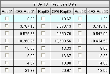
Replicate data column
CPS Column
Displays the CPS (counts per second) for each replicate data.
You can exclude unwanted replicate data from the analysis. To exclude replicate data, mark the check box next to the replicate data to ignore.

Conc. Column
Displays the concentration of the element in each replicate data set.
Customizing columns
Columns can be rearranged, added, and removed.
This section describes the customization procedure.
- Toggling between concentration and count view
- Rearranging columns
- Changing the column width
- Changing the column height
- Adding/Removing columns
- Displaying replicate data columns
- Restoring the default column settings
- Saving the column settings
- Loading the column settings
- Saving user-specific column settings
- Loading user-specific column settings
- Adjusting the column width to the text
- Fixing the Sample Columns
- Changing the ordering of analyte and ISTD columns
Toggling between concentration and count view
The icons on the toolbar when the layout is in “Table” mode let you toggle the view between concentration and count.

Rearranging columns
To rearrange the columns, follow these steps:
- Select the header for the column you want to move.
The entire column is selected.
- Drag the column header to the destination.
The column header moves, and red arrows are displayed at positions to which the column can be moved.
Moving a Column
- Release the mouse button at the destination.
The column moves to its new location.
Columns can also be rearranged using the context menu. For more information, refer to “Adding/Removing columns”.
Changing the column width
To change the column width, follow these steps:
- Place the mouse cursor at one border of the column you wish to
resize.
The cursor changes to
 .
. - Drag the cursor to change the column width.
To auto-adjust, double-click while
 is displayed.
Changing the column height
To change the column height, follow these steps:
- Place the mouse cursor on the leftmost column of the Batch Table.
The cursor changes to
 .
. - Drag the cursor to change the column height.
The new column height is applied to all the columns.
Adding/Removing columns
Columns can be added and removed from the Batch Table. Removing a column will not delete the associated data.
- Click [Add/Remove] from the [Columns] group on the [View] tab.
The [Add/Remove Columns] dialog box is displayed.
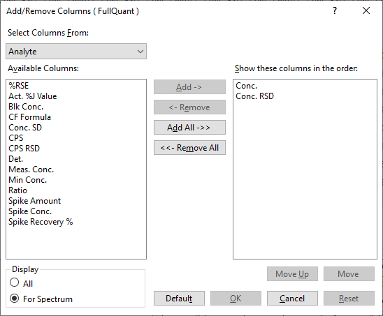
[Add/Remove Columns] Dialog Box
- From the [Select Columns From] list, select the category to add
columns to (or remove columns from).
You can select Sample, Analyte, ISTD, or Replicate Data columns.
- To add a column, select the columns to add from the [Available
Columns] list and click <Add->>.
The selected columns are added to the [Show these columns in the order] list.
To remove a column, select the column to remove from the [Show these columns in the order] list and click <<-Remove>.
The selected column is removed from the [Show these columns in the order] list.
- To change the display order of the columns, select a column from the [Show these columns in the order] list, and click <Move Up> or <Move Down> to change the order.
- When done, click <OK>.
The columns in the Batch Table are updated.
To restore the default column view, click  on the toolbar.
Displaying replicate data columns
While displaying a batch table in Table mode, you can display replicate data.
To display replicate data in the batch table, follow these steps:
- Click [Add/Remove] from the [Columns] group on the [View] tab.
The [Add/Remove Columns] dialog box is displayed.
- Select “Replicate data” from the [Select Columns From] list.
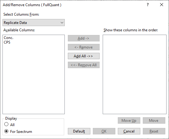
[Add/Remove Columns] Dialog Box
- Click [Add All ->>].
The selected columns will be added to the [Show these columns in the order] list.
- Click <OK>.
The replicate data will be displayed in the batch table.

You can exclude unwanted replicate data from the analysis. To exclude replicate data, click the checkbox next to the undesired replicate data.
To remove all replicate data from the selected samples, right-click the pane to display the context menu, select [Reject Settings]. When the [Reject Setting] dialog box, appears select the replicate data to remove.
To restore the default column view, click
on the toolbar.
Restoring the default column settings
To restore the default column settings after changing the types and ordering of the columns displayed, follow these steps:
- Click on the toolbar.
The default column settings are restored.
The width and height of the columns do not change.
Saving the column settings
Settings such as types and the order of the columns can be saved.
To save the current column settings, follow these steps:
When using ECM, OpenLab Server Products, Workstation Plus, or SDA, the displayed dialog box and the save file destination differ from standard MassHunter operations. For more information, refer to " Operations When Database Systems Are Used" in "Reference".
- Select [Load/Save] - [Save Columns Settings] from the [Columns]
group on the [View] tab.
The [Save As] dialog box is displayed.
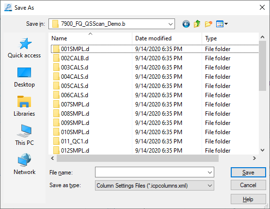
[Save As] Dialog Box
- Select the folder to save the settings in, enter a file name, and
click <Save>.
The column settings are saved.
Loading the column settings
To load the column settings that were saved in “Saving the column settings”, follow these steps:
When using ECM, OpenLab Server Products, Workstation Plus, or SDA, the displayed dialog box and the save file destination differ from standard MassHunter operations. For more information, refer to " Operations When Database Systems Are Used" in "Reference".
- Select [Load/Save] - [Load Columns Settings] from the [Columns]
group on the [View] tab.
The [Open] dialog box is displayed.
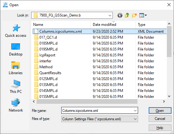
[Open] Dialog Box
- Select the folder where the column settings are saved, enter a
file name, and click <Open>.
The column settings are loaded, and the Batch Table is updated.
Saving user-specific column settings
This function is useful when a computer is shared between multiple users, or when the column settings are changed in the Data Analysis Method. Up to four sets of column settings can be saved. The saved column settings can be loaded easily from the toolbar.
To save the column settings for a specific user, follow these steps:
- Click [Settings] from the [Settings] group on the [Tools] tab.
[Settings] dialog box appears.
- Click [Edit] in “User Settings” from the [View] category.
The [Edit User Columns Settings] dialog box is displayed.
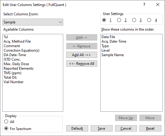
[Edit User Columns Settings] Dialog Box
- Under [User Settings], select the user (1 to 4) to edit the settings
for.
For information on other settings, refer to “Adding/Removing columns”.
- When done, click <OK>.
The columns in the Batch Table are updated.
To load user-specific column settings, refer to “Loading user-specific column settings“.
Loading user-specific column settings
To load user-specific column settings that were saved in the [Edit User Columns Settings] dialog box, click the corresponding icon on the toolbar.
 Displays the column settings saved
for “User Settings” “1”.
Displays the column settings saved
for “User Settings” “1”.
 Displays the column settings saved
for “User Settings” “2”.
Displays the column settings saved
for “User Settings” “2”.
 Displays the column settings saved
for “User Settings” “3”.
Displays the column settings saved
for “User Settings” “3”.
 Displays the column settings saved
for “User Settings” “4”.
Displays the column settings saved
for “User Settings” “4”.
To restore the default column view, click on the toolbar.
Adjusting the column width to the text
To automatically adjust the column width to fit the text, follow these steps:
- Click [Auto Fit] from the [Columns] group on the [View] tab.
All column widths are automatically adjusted to fit the text.
Fixing the Sample Columns
The Sample columns can be fixed so that they do not become hidden when you scroll to the right.
- Click [Lock Sample Columns] from the [Batch Table] group on the
[View] tab.
The Sample columns will be locked.
- To unlock the Sample columns, click [Lock Sample Columns] again.
When this command is highlighted, the Sample columns are locked. When this command is not highlighted, the columns are unlocked.
Changing the ordering of analyte and ISTD columns
By default, columns are displayed in the following order Analyte - ISTD and MS/MS Mass - Tune Modes However, this order can be changed. To change the order, follow these steps:
- Click [Arrange Elements] from the [Batch Table] group on the [View] tab.
- Select the order from the submenu.
- [Analyte - ISTD Order]: Displays in the Analyte - ISTD order.
- [ISTD - Analyte Order]: Displays in the ISTD - Analyte order.
- [Mass Order]: Displays in the Mass order.
- [Tune Mode - Mass Order]: Displays in the Tune Mode - Mass order.
- [MS/MS Order]: Displays in the MS/MS mass order.
- [Tune Mode - MS/MS Order]: Displays in the Tune Mode - MS/MS mass order.
The order of the columns in the Batch Table are updated. The order of the calibration curves on the Calibration Curve pane is also updated.
Sorting samples
The samples in the Batch Table can be sorted using the column headers. To sort the samples, follow these steps:
- Click the header of the column to sort by.
A arrow icon is displayed to the right of the column header, and the samples are sorted.
- The sort type (ascending or descending) switches when you click
the column header.
 : Descending order.
 : Ascending order.
To return to the default sort order, select [Reset Sort] from the context menu.
Switching the sample display setting
Samples that are displayed in the Batch Table can be shown or hidden.
- Showing/Hiding Based on the Outlier Type
- Showing/Hiding based on the sample type
- Showing/Hiding based on the tune mode
Showing/Hiding Based on the Outlier Type
You can show only the samples that have a specific outlier. You can also show only the samples that have no outlier.
To display the desired sample data, click on one of the following icons on the Batch Table pane toolbar.
 Displays samples
that have an outlier.
Displays samples
that have an outlier.
 Displays samples
that do not have an outlier.
Displays samples
that do not have an outlier.
To restore the view, click on the inverted outlier icon.
You can also click
 to open
the [FullQuant
Outliers] dialog box / [SemiQuant
Outliers] dialog box where you can select the type of outlier
to display in the Batch Table.
to open
the [FullQuant
Outliers] dialog box / [SemiQuant
Outliers] dialog box where you can select the type of outlier
to display in the Batch Table.
Showing/Hiding based on the sample type
You can show only the data for a specific sample type. To change the display, follow these steps:
- In the Batch Table pane toolbar, click the down arrow on
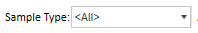 .
.
The [Sample Type] dialog box is displayed.
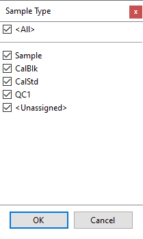
[Sample Type] Dialog Box
- Set the show/hide setting for each sample
type.
To show a sample type in the Batch Table, mark the corresponding check box. To hide the sample type, clear the check box.
- Click <OK>.
The selected sample types are displayed in the Batch Table. The ISTD Stability graph and QC Stability graph are also updated.
By default, all sample types are shown. To restore the default setting, check <All>.
Showing/Hiding based on the tune mode
If the sample was acquired in Multi Tune mode, you can elect to show only the data for a specific tune mode. To switch the display, follow these steps:
- In the Batch Table pane toolbar, click the down arrow on
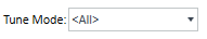 .
.
The list of tune modes is displayed.
- Select the tune mode to display.
The data for the selected tune mode is displayed in the Batch Table. The ordering of the calibration curves on the Calibration Curve pane will also be updated.
By default, data is shown for all tune modes. To restore the default setting, select <All>.
Displaying by calibration curve groups
To group and display the sample data by which calibration curve was used when using multiple calibration curves, follow these steps:
- Click [Group By Calibration] from the [Batch Table] group on the
[View] tab.
The sample data is grouped and displayed by calibration curve.
- To release grouping using the calibration curve, select [Group By Calibration] again.
Auto review
Auto review can be performed on the Batch Table for the samples or the elements.
Auto-reviewing the samples
When samples are auto-reviewed, the sample rows are automatically selected in sequence every few seconds. Auto-review starts with the selected (highlighted) sample row. The other panes (such as Spectrum pane and Calibration Curve pane) are automatically updated to match the selected sample. The auto review stops after the final sample in the Batch Table has been processed.
To perform an auto review of the samples, follow these steps:
- Click [Samples] from the [Auto Review] group on the [View] tab.
Auto review starts on the selected sample.
The [Auto Review] (Samples) dialog box is displayed.
[Auto Review] (Samples) Dialog Box
Auto review stops at the last sample row.
- To interrupt the auto review, click <Stop> in the [Auto
Review] (Samples) dialog box.
The auto review stops.
Auto-reviewing the elements
When elements are auto-reviewed, the element rows are automatically selected in sequence every few seconds. Auto-review starts with the selected (highlighted) element row. The other panes (such as Spectrum pane and Calibration Curve pane) are automatically updated to match the selected element. The auto review stops after the final element in the Batch Table has been processed.
To perform an auto review of the elements, follow these steps:
- Click [Elements] from the [Auto Review] group on the [View] tab.
Auto review starts on the selected element.
The [Auto Review] (Elements) dialog box is displayed.
[Auto Review] Dialog Box
Auto review stops at the last element row.
- To interrupt the auto review, click <Stop> in the [Auto
Review] (Elements) dialog box.
The auto review stops.
Exporting the batch table
The Batch Table can be exported in part or as a whole for use in other application.
- Exporting the entire table
- Exporting data for a selected area
- Transposing rows/columns and exporting
When using ECM, OpenLab Server Products, Workstation Plus, or SDA, the displayed dialog box and the save file destination differ from standard MassHunter operations. For more information, refer to " Operations When Database Systems Are Used" in "Reference".
Exporting the entire table
The Batch Table can be exported in its entirety. To export the whole Batch Table, follow these steps:
When using ECM, OpenLab Server Products, Workstation Plus, or SDA, the displayed dialog box and the save file destination differ from standard MassHunter operations. For more information, refer to " Operations When Database Systems Are Used" in "Reference".
- Right-click in the Batch Table.
The context menu is displayed.
- Select [Export] - [Export Table].
The [Export Table] (Entire Table) dialog box is displayed.
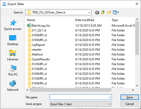
[Export Table] Dialog Box
- Select a folder to export the data to, and enter a file name.
- Select the export file type from the [Save as type] list.
- Excel File (*.xlsx)
- Excel 97-2003 File (*.xls)
- Comma-separated values File (*.csv)
- Tab Delimited File (*.txt)
- XML File (*.xml)
However, you can select an Excel file only when the Excel is installed.
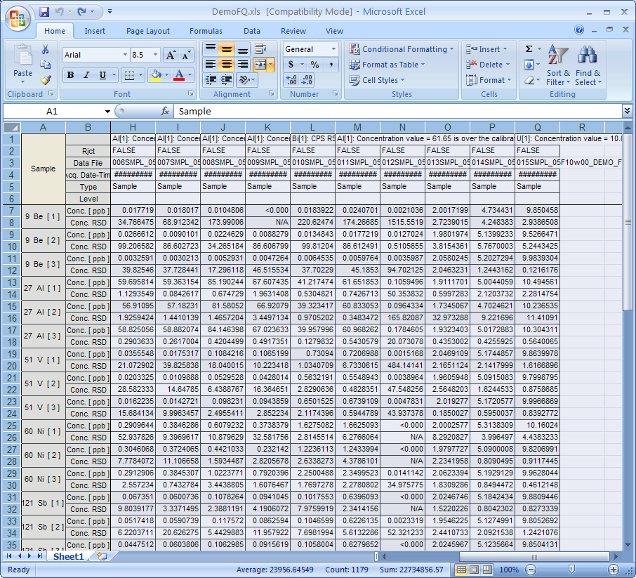
- Click <Save>.
Associated application starts, and then exported data is displayed.
It is always the acquired raw data that is exported regardless of the number of digits displayed.
You can edit, print, or save the data by using the functions of the associated application.
Exporting data for a selected area
The Batch Table can be exported partially by selecting the target area. To export data for the selected area only, follow these steps:
When using ECM, OpenLab Server Products, Workstation Plus, or SDA, the displayed dialog box and the save file destination differ from standard MassHunter operations. For more information, refer to " Operations When Database Systems Are Used" in "Reference".
- In the Batch Table, select the area for the data to be exported,
and right-click.
The context menu is displayed.
- Select [Export] - [Export Selected Area].
The [Export Table] (Area) dialog box is displayed.
[Export Table] Dialog Box
- Select a folder to export the data to, and enter a file name.
- Select the export file type from the [Save as type] list.
- Excel File (*.xlsx)
- Excel 97-2003 File (*.xls)
- Comma-separated values File (*.csv)
- Tab Delimited File (*.txt)
However, you can select an Excel file only when the Excel is installed.
- Click <Save>.
Associated application starts, and then exported data is displayed.
It is always the acquired raw data that is exported regardless of the number of digits displayed.
You can edit, print, or save the data by using the functions of the associated application.
Transposing rows/columns and exporting
You can transpose the rows/columns in the batch table and export it to a file.
The following file formats are available:
- Excel File (*.xlsx)
- Excel 97- 2003 File (*.xls)
- Comma- separated values File (*.csv)
- Tab Delimited File (*.txt)
However, you can select an Excel file only when the Excel is installed.
Transposing rows/columns and exporting to an Excel file
To transpose the rows and columns and export the batch table, follow these steps:
- Right-click on the Batch Table.
The context menu is displayed.
- Select [Export] - [Export Table with Transposition].
The exported data is opened in the associated application with the rows and columns transposed.
It is always the acquired raw data that is exported regardless of the number of digits displayed.
You can edit, print, or save the data by using the functions of the associated application.
Saving the batch result
This section explains how to save the current Batch Result.
When using ECM, OpenLab Server Products, Workstation Plus, or SDA, the displayed dialog box and the save file destination differ from standard MassHunter operations. For more information, refer to " Operations When Database Systems Are Used" in "Reference"".
Overwriting
To save the current Batch Result by overwriting, follow these steps:
When  is displayed, the file
cannot be saved. Click before
saving.
is displayed, the file
cannot be saved. Click before
saving.
- Click the [Save] from the [Batch] group on the [Home] tab.
The Batch Result will be overwritten.
Saving with a different name
To save the current Batch Result with a different file name, follow these steps:
When is displayed, the file
cannot be saved. Click before
saving.
- Select [Save] - [Save As] from the [Batch] group in the [Home]
tab.
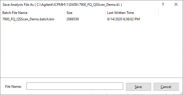
[Save Batch Result As] Dialog Box
- Enter a file name, then click [Save].
The Batch Result is saved under the specified file name.