Data Analysis for Chromatogram

In this section, data analysis procedure for a chromatogram is shown.

Opening the ICP-MSICP-QQQ Data Analysis window
Creating a batch folder
Loading the data
Sample type setup
Creating a chromatogram data analysis method
Executing analyses
Checking the analysis results
Saving the analysis results
Generating the Quick Batch Report
Generating the analysis results report
Closing the ICP-MSICP-QQQ Data Analysis window

MassHunter 5.2 or later comes with a Multi-Injection CIC function.

This function allows you to perform CIC (Compound Independent Calibration) by selecting a calibration analyte from two or more chromatographic injections.

Specifically, you can select the compound with a sample type of CICSpike as the calibrant (a point on the calibration curve) to allow quantification.

For details, refer to "MassHunter Workstation Chromatographic Software" manual.

Opening the ICP-MSICP-QQQ Data Analysis window

Open the [ICP-MSICP-QQQ Data Analysis] window to perform an analysis.

To open the [ICP-MSICP-QQQ Data Analysis] window, do the following step:

Click [Start] on the Windows taskbar and select [ICP-MSICP-QQQ MassHunter Workstation] >> [Offline Data Analysis], or double-click the shortcut icon on the Windows desktop.
The [ICP-MSICP-QQQ Data Analysis] window is displayed.

Creating a batch folder

Create a new batch folder by completing the following steps:

When using ECM, OpenLab Server Products, Workstation Plus, or SDA, the displayed dialog box and the save file destination differ from standard MassHunter operations. For more information, refer to "Operations When Database Systems Are Used" in "Reference".

Select [New Batch Folder] from the [File] tab and click [Browse].
The [New Batch Folder] dialog box is displayed.

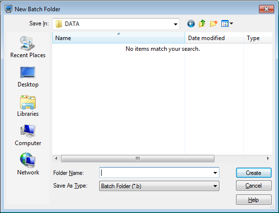
[New Batch Folder] Dialog Box
Open the folder you wish to create the batch folder in. Enter a folder name into the [Folder Name] text box, and click <Create>.
A Batch Folder for storing the analysis results is created.

Loading the data

Load the standard samples for the calibration curves and the unknown sample data into the Batch Table pane. You may also load the data after you create the Data Analysis Method.

To load the data, do the following steps:

Click [Import Samples] - [Import All Samples from Batch] from the [Batch] group on the [Home] tab.
The [Import All Samples from Batch] dialog box is displayed.

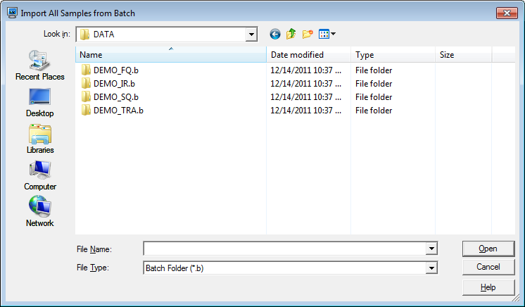
[Import All Samples from Batch] Dialog Box
Select a batch folder, and click <Open>.
The data is displayed in the Batch Table pane of the [ICP-MSICP-QQQ Data Analysis] window.

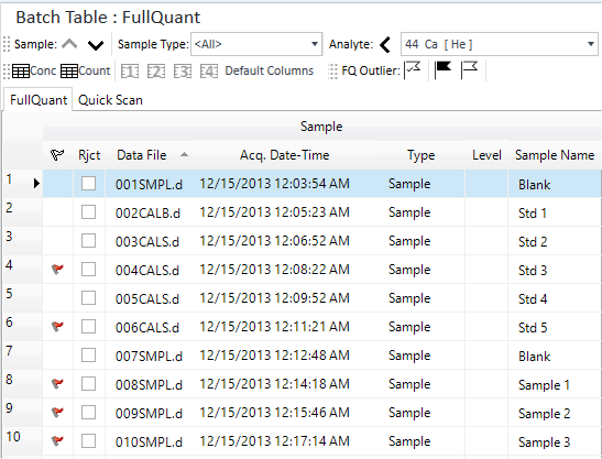
Batch Table Pane

Sample type setup

Specify the sample type and calibration curve level.

Change the settings for the Sample types that are displayed in the Type column of the Batch Table pane.

Standard sample for calibration curves: CalStd (set Level column to “1”, “2”, and “3” in ascending order of concentration)
Unknown sample: Leave as Sample

Creating a chromatogram data analysis method

Create a data analysis method by completing the following steps:

Click [Edit] from the [Method] group on the [Home] tab.
The [Method Editor] window is displayed.
Check that the Data Analysis Method table of the [Method Editor] window is configured as follows. If not, change the settings as necessary.
- [FullQuant Analysis] check box is marked.
- [Analysis Mode] is set to “Chromatogram”.
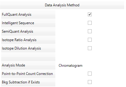
Data Analysis Method Table
In the Sample/Batch Template table of the [Method Editor] window, configure the template for the analysis result report.
There are two types of templates:
- Sample Template: Report of sample data
- Batch Template: Report of the entire batch
Click the on the right end of the box to select a template, as necessary.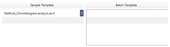

Sample/Batch Template Table

The rows of the Sample/Batch Template table correspond to the rows of the Data Analysis Method table. Specify a template in the box on the same row of the selected Data Analysis Method.
For more information, refer to “Sample/Batch Template table”.

From the Method Development Tasks pane, click [Open standard data file].
The [Select Data] dialog box appears.

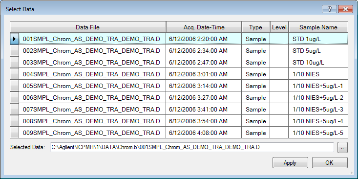
[Select Data] dialog box

Select calibration curve data and click <Apply>.
The Chromatogram pane displays the peaks for calibration curves.
Select a suitable data for calibration curves, and then click [OK].
The Integration Parameters Pane and Chromatogram pane (Method Editor) are displayed.
From [TIC/EIC] List in the Toolbar on the Chromatogram Pane, select the mass of the analytes.
The lower part of the Chromatogram pane shows the Chromatogram of the standard data for the selected element.

The peaks that are included in the autointegration are displayed in green and the peaks that are not displayed in the peak list are displayed in purple. Also, the peaks that are not included in the autointegration are displayed in white. The baseline is displayed in red.

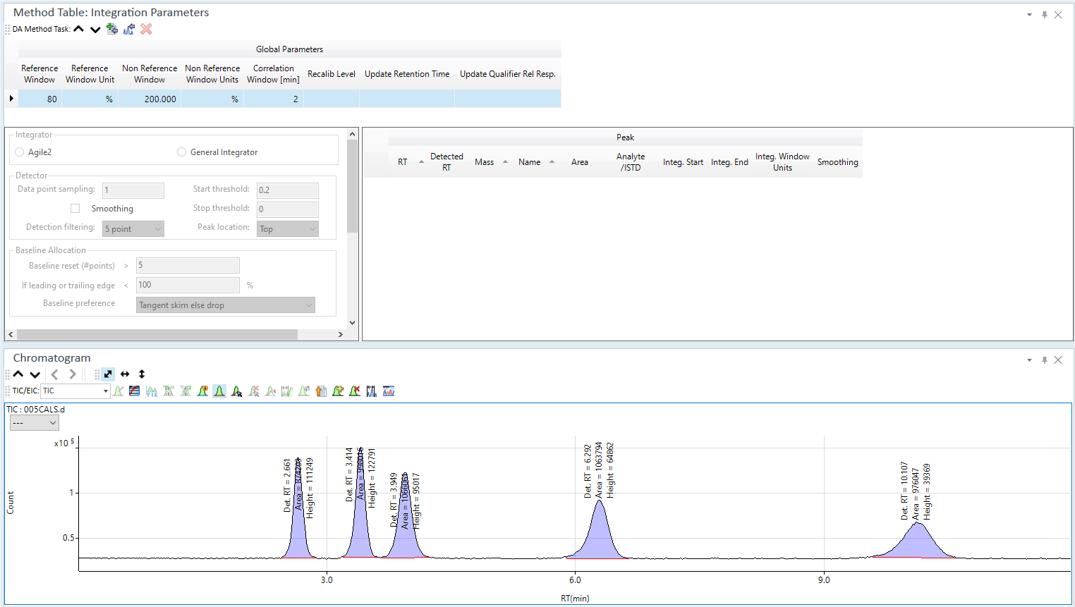
Integration Parameters Pane and Chromatogram Pane (Method Editor)

If the Chromatogram pane (Method Editor) is not displayed, click [Panes] from the [Show] group on the [View] tab.

To add peaks in the Peak List Table, complete the following steps:
(1) Click on the toolbar in the Chromatogram Pane.

(2) When the cursor shape changes to , click the peaks to add.

The data of the added peaks are added to the Peak List Table.

(3) When you have added the peaks, click again.

To delete peaks, click . When the cursor shape changes to , click the peaks you want to delete. After you delete the peaks, click again.
To add all peaks, click on the toolbar.

To add peaks that are not detected with the default integration parameters, complete the following steps:

To add peaks after you change the integration parameters of each peak or those of the entire chromatogram

(1)   Change the integration parameters of each peak or those of the entire chromatogram in the Integration Parameters Table, as needed.

(2)   After the peaks are found, click on the toolbar in the Chromatogram Pane.

(3)   After the cursor shape changes to , click the peaks to add.

   The data of the added peaks are added to the Peak List Table.

(4)   After you add the peaks, click again.

To add peaks after you specify an integration range

(1)   Click on the toolbar in the Chromatogram Pane.

(2)   After the cursor shape changes to , drag to specify the range that contains the peaks to add.

(3)   In the Integration Parameters Table, change the integration parameters for the selected area.

(4)   After the peaks are found and displayed in blue, click the [Reintegrate] button.

(5)   Click .

(6)   After the cursor shape changes to , click the peaks to add.

   The data of the added peaks are added to the Peak List Table.

(7)   After you add the peaks, click again.

Integration Parameters pane

The Integration Parameters pane displays the following tables. For more information about settings, refer to the following topics:

The Peak List Table lets you do the following operations.

When a peak line is selected, the corresponding peak is highlighted in the Chromatogram pane (Method Editor)
Clicking the header for the mass column sorts the elements by mass number.
To delete rows, select the row to delete, then right-click on the cell at the beginning of the row and click [Delete] from the context menu.
To delete a group of consecutive rows, click on the first row, then hold the Shift key and click on the last row.
The RT for all analytes can be shifted if necessary, such as when a column ages. Right-click on the table and select [Shift Retention Time] from the context menu, then enter the shift value in the [Shift Retention Time] dialog box.

In the Method Development Tasks pane, click [FullQuant].
The Calibration pane is displayed.

Specify the formula for the calibration curve and the concentration of the calibration curve level.

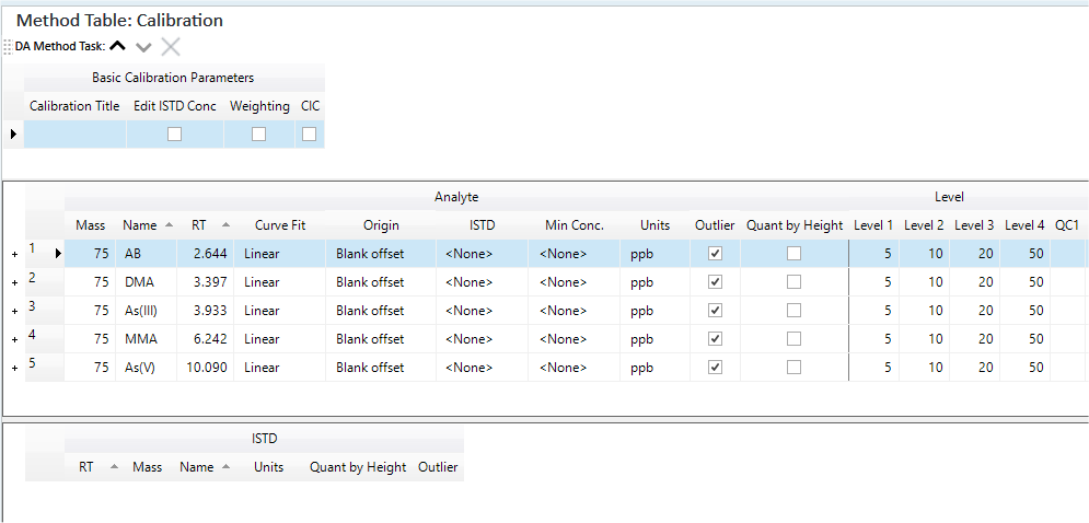
Calibration Pane

For information about these settings, refer to “Calibration pane”.
Configure the following settings as necessary:
- To set the Outlier conditions:
  In the Method Development Tasks pane, click [QC Setup]. The FullQuant Outlier Setup pane is displayed, which lets you set the outlier conditions.
  
  For information about these settings, refer to “FullQuant Outlier Setup pane”.
- To set a Worklist, configure custom actions and auto-saving of an analysis results report:
  In the Method Tasks pane, click [Worklist Actions].
  
  The Work List Actions pane is displayed, which lets you set up the Worklist.
  
  For information about these settings, refer to “Work List Actions pane”.
When you have created or changed the data analysis method, click [Validation] in the Method Development Tasks pane.
If an error is found in the data analysis method, the error information is displayed in the Method Error List pane. Fix the errors.

If no error is found, a confirmation dialog box is displayed.

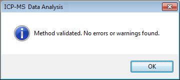
Confirmation Dialog Box
Click <OK>.
In the Method Development Tasks pane, select [Return to Batch List].
When asked whether to save the Data Analysis Method, click <Yes>.
Proceed to the analysis process.

Executing analyses

To perform an analysis, complete the following step:

Click [Process Batch] from the [Batch Option] group on the [Home] tab.
An analysis is performed using the settings defined by the Data Analysis Method, and the analysis results are displayed in the Batch Table pane.

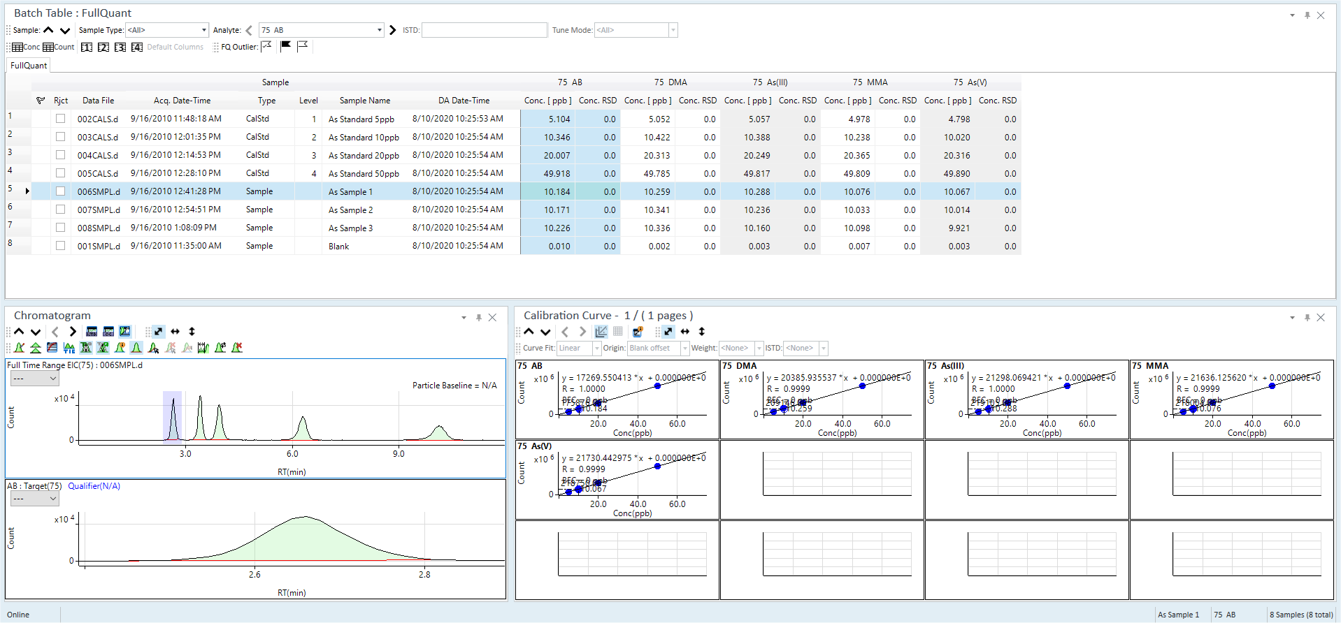
Analysis Results

Proceed to checking and correcting the analysis results.

To clear the analysis results, click [Clear Results] - [Clear Results] from the [Batch Option] group on the [Home] tab. If the data or the Data Analysis Method has been changed, repeat the analysis.

Checking the analysis results

This section describes the procedures for checking and correcting the analysis results.

Checking the Batch Table pane

The Batch Table pane displays the concentration and concentration RSD for each peak in the samples.

For more information on how to view and use the Batch Table pane, refer to “Batch Table Pane Operation”.

On chromatograms, the area value is displayed as "count". Therefore, "count" and "area" represents the same thing. Also, the "count" is used in quantification.

For Chromatogram analysis before MassHunter 5.1, the concentration results in the Batch Table are calculated based on the count rounded after the decimal point.
On the other hand, the “Calc Conc.” results for the Calibration table in the Calibration Curve pane are calculated based on counts that are not rounded.
From MassHunter 5.2, both are calculated using non-rounding counts. Due to the change in the calculation method, if the analysis results from MassHunter 5.1 or earlier are read in 5.2, you need to perform batch processing again.

Checking the Chromatogram pane

The Chromatogram pane (Option) displays the chromatogram peaks.

For more information on how to view and use the Chromatogram pane (Option), refer to “Chromatogram Pane Operations”.

Checking the Calibration Curve pane

The Calibration Curve pane displays the calibration curves for each element in the samples.

For more information on how to view and use the Calibration Curve pane, refer to “Calibration Curve Pane Operation”.

Checking the ISTD Stability Graph pane

When using internal standard correction, the recovery (%) of each ISTD element is displayed in the ISTD Stability Graph pane. Recovery values less than 100% may indicate that the analysis result is less reliable.

For more information on how to view and use the ISTD Stability Graph pane, refer to “ISTD Stability Graph Pane Operation”.

Saving the analysis results

For more information, refer to “Saving the analysis results” under “Common Data Analysis Operations”.

Generating the Quick Batch Report

To print a summary of the analysis results, print a Quick Batch Report. For more information, refer to “Generating the Quick Batch Report” under “Common Data Analysis Operations”.

Generating the analysis results report

For more information, refer to “Generating the analysis results report” under “Common Data Analysis Operations”.

Closing the ICP-MSICP-QQQ Data Analysis window

For more information, refer to “Closing the Data Analysis window” under “Common Data Analysis Operations”.